Name the case first (worst, average, best, or amortized), then give the tightest bound you can justify. “Worst case Θ(n²), expected Θ(n log n)” says more than “O(n²),” and it shows you know the difference between choosing inputs and bounding a function.
What Big O actually says
NIST's Dictionary of Algorithms and Data Structures gives the formal version: f(n) = O(g(n)) means there are positive constants c and k such that 0 ≤ f(n) ≤ c·g(n) for every n ≥ k. It is an upper bound, up to a constant factor, for large enough n. Ω is the matching lower bound, and Θ means both at once: f is squeezed between two constant multiples of g.
Two consequences surprise people. First, Big O is about growth, not speed: an O(n) function with a large constant can lose to an O(n²) one on small inputs. Second, an upper bound can be loose. Linear search is technically O(n²), because n ≤ n², but no interviewer would accept that answer. In conversation “O” usually means the tightest bound you can prove, so give the tight one.
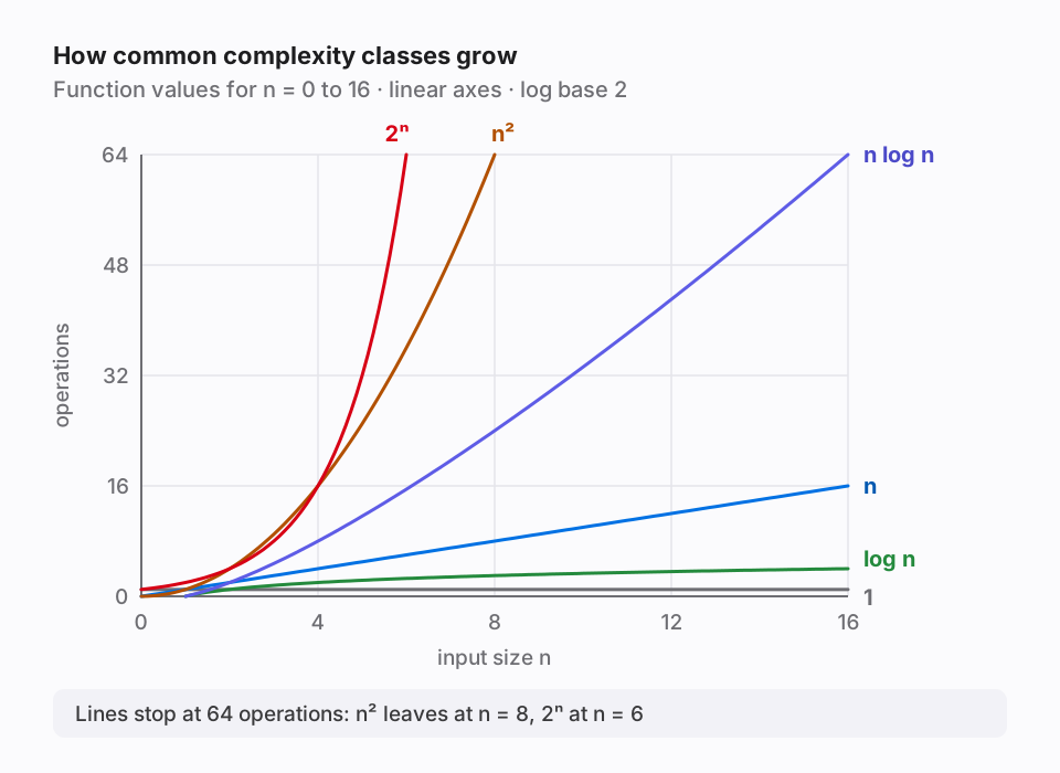
Big O graph: how the common classes grow
The chart plots each function with log base 2 and no constant factors. At n = 4, n² and 2ⁿ are both 16 and n log n is 8, so small inputs make the classes look alike. By n = 8, n² has reached 64 and 2ⁿ is already 256. The table pushes n to 1,000, where the differences stop being visual and become questions of feasibility.
Read the n = 1,000 column as a rough count of basic steps. An n log n sort does about ten thousand, an n² double loop does a million, and a brute force over all subsets would need about 1.07 × 10³⁰¹ steps, which no hardware finishes. That is why interviewers push from O(2ⁿ) to a polynomial dynamic program, and from O(n²) to O(n log n) or O(n), before they care about constants.
| Class | Typical code | n = 10 | n = 1,000 |
|---|---|---|---|
| O(1) | Index into a list | 1 | 1 |
| O(log n) | Binary search | 3.3 | 10 |
| O(n) | One pass | 10 | 1,000 |
| O(n log n) | Comparison sort | 33 | 9,966 |
| O(n²) | All pairs | 100 | 1,000,000 |
| O(2ⁿ) | All subsets | 1,024 | ≈ 1.07 × 10³⁰¹ |
Derive complexity from code: loops, nesting, halving
Counting beats pattern-matching. The script counts iterations for four shapes: a single loop, a nested loop over the full range, a nested loop whose inner range starts at i + 1, and a loop that halves m until it reaches 1. Doubling n doubles the first count, quadruples the second, roughly quadruples the third, and adds one to the last. Those ratios are the fingerprints of O(n), O(n²), O(n²), and O(log n).
For n = 64 the output is (64, 4096, 2016, 6). The triangle loop does n(n − 1)/2 = 2,016 iterations, half of the full nested loop, but a half is a constant factor, so it is still Θ(n²). The rules follow: sequential blocks add, so O(n) + O(n²) is O(n²); nested loops multiply when their bounds are independent; a loop that divides its range by a constant runs Θ(log n) times.
def count_ops(n):
    single = sum(1 for _ in range(n))
    nested = sum(1 for _ in range(n) for _ in range(n))
    triangle = sum(1 for i in range(n) for _ in range(i + 1, n))
    halving, m = 0, n
    while m > 1:
        m //= 2
        halving += 1
    return single, nested, triangle, halving

for n in (8, 16, 32, 64):
    print(n, count_ops(n))
Recursion trees: n log n versus exponential
For recursion, write the recurrence and add up the work per level. Merge sort splits the input in half and merges in linear time: T(n) = 2T(n/2) + n. Each level of the recursion tree does n work in total and there are log₂ n levels, so the total is n log n, as MIT's 6.006 lecture notes also state. The script confirms it exactly for powers of two: 24 for n = 8, 384 for 64, and 10,240 for 1,024.
Naive Fibonacci also makes two calls, but each shrinks n by only one or two, so the tree stays deep and bushy. The script counts 177 calls for n = 10, 21,891 for n = 20, and 242,785 for n = 25, about 1.6 times more per step: exponential growth. Space behaves differently. The recursion is never more than n frames deep, so the stack is O(n) even while the call count explodes.
def merge_work(n):        # T(n) = 2T(n/2) + n, like merge sort's merging
    if n <= 1:
        return 0
    return 2 * merge_work(n // 2) + n

calls = 0
def fib(n):               # T(n) = T(n-1) + T(n-2) + 1: naive recursion
    global calls
    calls += 1
    return n if n < 2 else fib(n - 1) + fib(n - 2)

for n in (8, 64, 1024):
    print("merge", n, merge_work(n))
for n in (10, 20, 25):
    calls = 0
    fib(n)
print("fib", n, calls)Best, average, and worst case are not O, Θ, and Ω
A common confusion maps worst case to O, best case to Ω, and average case to Θ. These are independent questions. The case picks which inputs you measure: the worst input of size n, the best one, or an average over a stated distribution. The bound says how tightly you have pinned down the cost for that case. Insertion sort's worst case is Θ(n²) and its best case, an already sorted array, is Θ(n); both are exact statements.
Quicksort is the example interviewers like. NIST lists its running time as Θ(n²) in the worst case while it is typically O(n log n), so “quicksort is O(n log n)” is false as a worst-case claim. Hash tables are similar: the Python documentation lists dict and set lookups as O(1) on average and notes that they become O(n) when every key hashes to the same value.
| Algorithm | Best case | Average case | Worst case |
|---|---|---|---|
| Linear search | Θ(1) | Θ(n) | Θ(n) |
| Binary search | Θ(1) | Θ(log n) | Θ(log n) |
| Insertion sort | Θ(n) | Θ(n²) | Θ(n²) |
| Quicksort | Θ(n log n) | Θ(n log n) | Θ(n²) |
| dict lookup in CPython | O(1) | O(1) | O(n) |
Amortized cost and a Python cheat sheet
Python's design FAQ explains that CPython lists are variable-length arrays and that, when the array must grow, extra space is allocated so the next few appends need no resize. An append that triggers a resize copies every element, an O(n) step; amortized analysis spreads that cost over the cheap appends around it. The script watches sys.getsizeof over 64 appends and, on CPython 3.12 and 3.14 on macOS, prints [1, 5, 9, 17, 25, 33, 41, 53]: only eight resizes. The exact points are a CPython implementation detail.
The table comes from the official Python page on time complexity of built-in types, which replaced the long-cited Python wiki TimeComplexity page and describes CPython. The deque row comes from the collections documentation. Space deserves the same scrutiny: a[i:j] copies j − i references, recursion holds a frame per level, and sorted() returns a new list while list.sort() works in place.
import sys

a, grew_at, last = [], [], sys.getsizeof([])
for i in range(64):
    a.append(i)
    size = sys.getsizeof(a)
    if size != last:          # capacity changed: the array was resized
        grew_at.append(len(a))
        last = size
print(grew_at)
print(len(grew_at), "resizes in", len(a), "appends")| Operation | Cost | Note |
|---|---|---|
| list.append(x) | O(1) | Amortized; a resize is O(n) |
| list.insert(0, x), list.pop(0) | O(n) | Shifts every element |
| x in list | O(n) | Linear scan |
| x in set, d[key] | O(1) | Average; O(n) worst case |
| deque.appendleft, deque.popleft | O(1) | Use instead of list.pop(0) |
| list.sort(), sorted() | O(n log n) | O(n) comparisons on sorted input |
How to answer a complexity question in an interview
Use a fixed script. Name the size variables (n items, m edges, k window), state the case, give time and then extra space, and point at the line that dominates: “Worst case O(n log n) for the sort on line two; the loop after it is O(n); O(n) extra space for the sorted copy.” If the input has two sizes, keep both. A graph traversal is O(n + m), not O(n).
Common mistakes: dropping the log factor of a sort, calling a frequency map O(1) space because the alphabet is fixed without saying so, building a string by concatenation in a loop (the Python docs call this quadratic in total length), and quoting amortized costs as per-call guarantees. Practice with the question sets below until the table above is automatic.
Quick answers
Frequently asked questions
What is the difference between O(n) and Θ(n)?
O(n) promises the cost grows no faster than a constant times n. Θ(n) promises it grows exactly that fast, within constant factors, from above and below. A Θ(n) function is also O(n) and O(n²), but only the Θ statement is tight.
Is O(2n) different from O(n)?
No. The constant c in the definition absorbs constant factors, so O(2n), O(n + 100), and O(n) describe the same set of functions. Mention a constant in your explanation when it matters for practical speed, but drop it in the notation.
Does Big O apply to space as well as time?
Yes, the same definition bounds memory as a function of input size. Interviewers usually mean auxiliary space, the memory allocated beyond the input: O(1) for in-place two pointers, O(n) for a hash set or memo table, O(depth) for recursion.
Why is dict lookup called O(1) if the worst case is O(n)?
The O(1) figure is an average case that assumes keys hash well and collisions are rare. The Python documentation states that if every key hashed to the same value, each of those operations would take O(n). Say “average O(1)” in interviews.
Source notes
References and review policy
Information checked on November 7, 2026. Section links identify sources for factual claims and technical explanations. Interpretations, practice scenarios and preparation recommendations are RecallDeck’s editorial work.
- NIST Dictionary of Algorithms and Data Structures: big-O notation
- NIST Dictionary of Algorithms and Data Structures: quicksort
- Python docs: Time complexity of operations on built-in types
- Python design FAQ: How are lists implemented in CPython?
- Python docs: collections.deque
- MIT 6.006 (Spring 2020) Lecture 15 notes: Recursive Algorithms, SRTBOT
From reading to recall
Practice the full interview loop.
RecallDeck schedules the concepts you miss and keeps coding, design, and behavioral fundamentals available when the interviewer changes direction.